Computing Block-wise Cross Correlation

The cross correlation of two vectors using discrete Fourier transform (DFT) is a popular method of searching the occurrences of one pattern inside another. It provides simple mean to detect echoes, specific patterns inside digital signals, signal comparison etc.

In some applications, one of the input vectors (signals) is much longer than another, or even of infinite length. For example: searching a transmitted signal’s echo in the received input stream in radar or sonar, or detecting an RDS signal inside a continuous radio transmission. In such applications one must compute the cross correlation of searched pattern and input stream in a block-by-block manner.

In this article I shall present a short MATLAB template to compute a block-wise cross correlation appropriate for searching a specific pattern vector inside a continuous input vector of indefinite size. Furthermore, I shall extend the algorithm to search for more pattern vectors simultaneously.

Single pattern vector, single input vector

Explaining the entire theory of DFT and cross correlation is beyond the scope of this article. So let us skip to the algorithm itself. Define:

• M as the length in samples of pattern vector sought.
• N as the length in samples of DFT our hardware is able to perform. Must be bigger than 2×M-2. Bigger the number N, less computational overhead we get. Keep it a power of two to take advantage of FFT.
• N_n as the maximum length of block in samples. It equals to N-2×M+2.

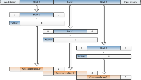
The algorithm is using the “overlap and add” technique to compute cross correlation of each block the following way:

1. Take N_n samples of the input vector. Pad it with zeros to cancel the periodic effect at both edges of cross correlation and to make it N samples long.
2. Pad the pattern vector with zeros to make it N samples long.
3. Compute cross correlation using FFT.
4. Overlap and add first M-1 samples of cross correlation with the end of the cross correlation of the previous block. This corrects the effect of neighbouring blocks.
5. The first N_n samples of the result is the final cross correlation (delayed by M-1 samples). Process the result accordingly.
6. Store the last M-1 samples of cross correlation for the overlap and add with the cross correlation of the next block.

Figure 1: Block-wise cross correlation computation

Note that we can prepare pattern vector’s DFT conjugate in advance to speed up the computation of cross correlation. See the Figure 1 above to get the general idea, how to iterate the process. Below is the example in MATLAB.

% Block-wise Cross Correlation
%
%   Input:
%      N      - Maximum block size (bigger performs more efficiently,
%               smaller uses less memory). Should be a power of two to make
%               use of FFT. Must be greater than twice the size of the
%               pattern vector minus one.
%      x_p    - The pattern vector to compute cross correlation with the
%               input vector.

%   Copyright 2012 Simon Rozman.

% TODO: Replace input data with actual block size and pattern vector.
N = 1024;
x_p = random('unif', -1.0, 1.0, 15, 1);

% Precompute pattern vector's DFT conjugate.
M = length(x_p);
X_p = conj(fftr([x_p; zeros(N - M, 1)]));

% N_n is the maximum "effective" block length of input vector to compute
% correlation.
N_n = N - 2*M + 2;

% Initialize a buffer to hold the intermediate samples for overlap add.
r_prev = zeros(M - 1, 1);

while 1
    % Read N_n samples of input vector. Store the number of samples actualy
    % read to N_read.
    %
    % TODO: Replace random generator with reading of the input vector.
    x = random('unif', -1.0, 1.0, N_n, 1);
    N_read = length(x);
    if N_read < 1
        break;
    end

    % Prepend M - 1 zeros, to make space for intermediate samples of
    % current block correlation to the previous block correlation effect.
    %
    % Append at least M - 1 zeros, to make space for intermediate samples
    % of current block correlation to the next block correlation effect,
    % and to extend the block to N samples.
    %
    % Compute FFT of the extended block.
    X  = fftr([zeros(M - 1, 1); x; zeros(N - M - N_read + 1, 1)]);

    % Calculate correlation between extended block and pattern vector.
    rr = ifftr(X .* X_p);

    % Overlap and add the intermediate samples from the previous block
    % (first M - 1 samples of extended block correlation).
    rr(1:(M - 1)) = rr(1:(M - 1)) + r_prev;

    % We finalized the next N_read samples of the result now. However,
    % delayed by M - 1 samples.
    %
    % TODO: Process the resulting correlation.
    plot(rr(1:N_read));

    % Store the ending M - 1 intermediate samples of the correlation to be
    % overlaped and added to the next block.
    r_prev = rr((N_read + 1):(N_read + M - 1));
end

Multiple pattern vectors, single input vector

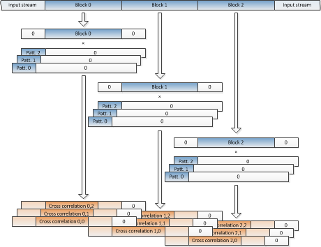
When searching for more than one pattern vector, we can save some time by reusing the FFT of input vector block already computed when computing the cross correlation with the first pattern vector. Providing that the pattern vectors are of similar, but not necessary the same length. M is the length in samples of the longest pattern vector sought now. From here on, N and N_n are defined the same way as before.

The algorithm is extended to minimize the number of required DFTs when computing the cross correlations. It pre-computes the DFT conjugates of pattern vectors as did the single pattern vector version before.

Figure 2: Block-wise multiple cross correlation computation

% Multiple Block-wise Cross Correlation
%
%   Input:
%      N        - Maximum block size (bigger performs more efficiently,
%                 smaller uses less memory). Should be a power of two to
%                 make use of FFT. Must be greater than twice the size of
%                 the longest pattern vector minus one.
%      patterns - Table of pattern vectors to compute cross correlation
%                 with the input vector.

%   Copyright 2012 Simon Rozman.

% TODO: Replace input data with desired block size and pattern vectors.
N = 1024;
patterns(1).x = random('unif', -1.0, 1.0, 15, 1);
patterns(2).x = random('unif', -1.0, 1.0, 20, 1);
patterns(3).x = random('unif', -1.0, 1.0, 12, 1);

% Number of pattern vectors we're computing correlation of the input vector
% with.
P = length(patterns);

% Determine M: the length of the longest pattern vector measured in
% samples. Also, precompute all pattern vectors's DFTs conjugates.
M = 0;
for p = 1:P
    patterns(p).M = length(patterns(p).x); %#ok<*SAGROW>
    patterns(p).X = conj(...
        fftr([patterns(p).x; zeros(N - patterns(p).M, 1)]));
    M = max([patterns(p).M; M]);
end

% N_n is the maximum "effective" block length of input vector to compute
% correlation.
N_n = N - 2*M + 2;

% Initialize a buffer to hold the intermediate samples for overlap add.
r_prev = zeros(M - 1, P);

while 1
    % Read N_n samples of input vector. Store the number of samples actualy
    % read to N_read.
    %
    % TODO: Replace random generator with reading of the input vector.
    x = random('unif', -1.0, 1.0, N_n, 1);
    N_read = length(x);
    if N_read < 1
        break;
    end
    
    % Prepend M - 1 zeros, to make space for intermediate samples of
    % current block correlation to the previous block correlation effect.
    %
    % Append at least M - 1 zeros, to make space for intermediate samples
    % of current block correlation to the next block correlation effect,
    % and to extend the block to N samples.
    %
    % Compute FFT of the extended block.
    X  = fftr([zeros(M - 1, 1); x; zeros(N - M - N_read + 1, 1)]);
    
    for p = 1:P
        % Calculate correlation between extended block and each individual
        % pattern vector.
        rr = ifftr(X .* patterns(p).X);

        % Overlap and add the intermediate samples from the previous block
        % (first M - 1 samples of extended block correlation).
        rr(1:(patterns(p).M - 1)) = ...
            rr(1:(patterns(p).M - 1)) + r_prev(1:(patterns(p).M - 1), p);
        
        % We finalized the next N_read samples of the result now. However,
        % delayed by M - 1 samples.
        %
        % TODO: Process the resulting correlation.
        subplot(P, 1, p);
        plot(rr(1:N_read));
        
        % Store the ending M - 1 intermediate samples of the correlation to
        % be overlaped and added to the next block.
        r_prev(1:(patterns(p).M - 1), p) = ...
            rr((N_read + 1):(N_read + patterns(p).M - 1));
    end
end

Requirements

1. FFTR and IFFTR functions described here. When computing cross correlation of complex vectors, replace them with MATLAB’s built-in functions FFT and IFFT accordingly.